3.0 Generate possible intervention combinations
In this section, we describe the method for creating all possible combinations of the 16 public health interventions selected from the the CDC’s Compendium of Evidence-Based Interventions and Best Practices for HIV Prevention (Project, n.d.) using the scale.interventions.combination function in LEMHIVpack. See Figure 3 below for the list of interventions and their respective categories (Protect, Diagnose, Treat). We excluded combinations that would not be practically implemented jointly, termed “mutually exclusive combinations” (e.g. two HIV testing interventions delivered in primary care).
\(~\)
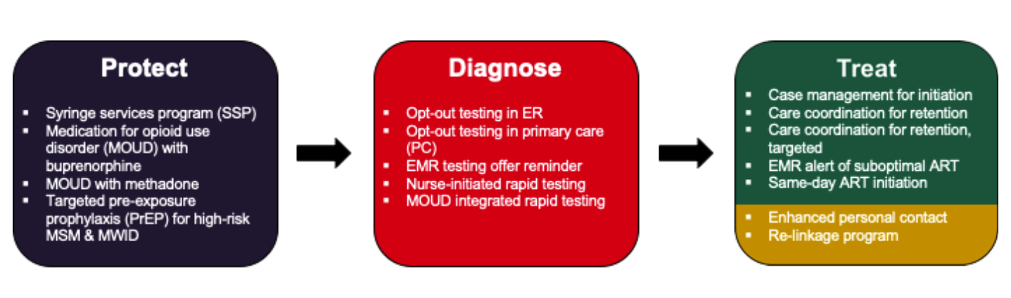
Figure 3.0 Evidence based interventions selected from the the CDC’s Compendium of Evidence-Based Interventions and Best Practices for HIV Prevention
\(~\)
Next, we set intervention parameters using the intervention.model.combination function, and then use the scale.interventions.combination function to calculate the scale of delivery inputs at each time step. Both are included in LEMHIVpack and the code can be found in the R directory of the github repository. Recall that scale refers to the proportion of a target population that is provided with an intervention. For HIV prevention programs, scale of delivery was the annual rate of expanded access, or additional scale-up, estimated using the best-available program-specific evidence. In contrast, for HIV testing and care interventions, scale of delivery was defined as the product of setting specific reach and adoption for each intervention i, target population j and healthcare setting k, where reach is defined as the participation rate in a given intervention, conditional on the probability an individual will access services in setting k and the probability the individual will accept the intervention being delivered.
\[Scale_{i,j} = reach_{j,k} \times adoption_{i,k}\]
\(~\)
To set indicators of modifying parameters in ODE model we use the function true.false.interventions.combination.
\(~\)
3.1 Derive intervention scale-up
In this component we derive the scale of delivery (or scale-up) of interventions, implemented proportionally across groups, for each time step. Some parameters and interventions only had evidence and input data stratified by race and sex (i.e. opt-out testing in ER) while others were stratified by race, sex and risk group (i.e. same-day ART initiation). Table 3.0 specifies how interventions were stratified; note that how an intervention was stratified is a result best available evidence as detailed in our previous manuscript (Krebs et al. 2020). Use set.scale.race.gender and set.scale.risk.race.gender to derive scale-up for interventions. In these scripts, matrices for scale estimates (with upper and lower bounds) are created; they each have 19 rows (one for each model compartment/state) and 42 columns (one for each population strata).
\(~\)
Table 3.0: Stratification of interventions input data
| Stratified by | Interventions |
|---|---|
| Race, Sex | Diagnose |
| * Opt-out testing in ER | |
| * Opt-out testing in primary care | |
| * Nurse initiated rapid testing | |
| * Emr testing offer reminder | |
| Race, Sex, Risk Group | Protect |
| * Syringe Service Program (SSP) | |
| * Medication for opioid use disorder (MOUD) with buprenorphine | |
| * Medication for opioid use disorder (MOUD) with methadone | |
| * Targeted PrEP for high-risk MSM and MWID | |
| Diagnose | |
| * MOUD integrated rapid testing | |
| Treat | |
| * Individual case management for ART initiation initiation | |
| * Individual care coordination for ART retention | |
| * Individual care coordination for ART retention, targeted | |
| * EMR alert for suboptimal ART engagement | |
| * Rapid/Same-day ART initiation | |
| * ART Re-engagement - Enhanced personal contact | |
| * ART Re-linkage program |
\(~\)
3.2 Model outcomes
In this component we run several R scripts that set up the production of model outcomes for output to excel. Model projected outcomes such as incremental and total costs (2018 USD) and QALYs gained are produced for each city, for the combinations of interventions, considering implementation and sustainment periods determined in Section 3.1.
Point estimates, and upper and lower bounds for estimates are first organized in arrays using accumulate.outcomes.combination. The number of infections for a given year (annual incidence rate) and cumulatively over several time horizons (5, 10, 20 years) are calculated for each city using time.period.infections. Both sets of output results (costs and QALYs, and number of infections) can then be exported to excel using CascadeCEA-Interventions-0-Output-write.excel.R. Lastly, population lists and number of infections for each time step, cost-effectiveness analyses results etc. are calculated and aggregated using the comb.eva.func.R function.
\(~\)
References
Krebs, E., X. Zang, B. Enns, J. E. Min, C. N. Behrends, C. Del Rio, J. C. Dombrowski, et al. 2020. “The Impact of Localized Implementation: Determining the Cost-Effectiveness of Hiv Prevention and Care Interventions Across Six United States Cities.” Journal Article. AIDS 34 (3): 447–58. https://doi.org/10.1097/QAD.0000000000002455.
Project, HIV/AIDS Prevention Research Synthesis. n.d. “Compendium of Evidence-Based Interventions and Best Practices for Hiv Prevention.” Report. Centers for Disease Control and Prevention. https://www.cdc.gov/hiv/research/interventionresearch/compendium/index.html.